This lab introduces some of the tools used with raster data. Rasters are appropriate for quantities that vary continuously and rapidly in space, in particular elevation and slope. In ArcGIS these tools are part of the Spatial Analyst extension.
We start by interpolating elevation from the discrete set of points in the spots
data set, which contains the vertices of contour lines from the USGS topographic
map, according to its metadata.
|
(note: the topo map and spots dataset shown here are both in NAD1927 coordinate system, from a previous lab; the current lab uses the spots dataset transformed to NAD1983.) |
|
|
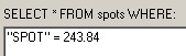
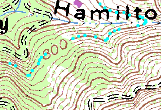
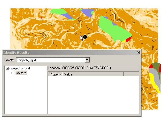
These contour lines were originally drawn from pairs
of aerial photographs viewed with a stereoscope. The
elevation has apparently been converted from feet to meters: in the image above,
the elevation of the selected spots is 800 feet = 243.84 meters.
There are various methods of interpolating between irregularly spaced points.
We'll use a tension spline. ArcMap creates a raster with the requested cell size
of 20 feet. The
individual cells, interpolated between the spots, can be seen in this snapshot of another part of the map:
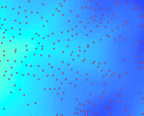
(Notes on displaying raster: To show the discreteness of the cells, the map is
zoomed in so each cell takes up 10 screen pixels, and the display is set to
"nearest neighbor" in the Display tab of the Layer Properties dialog.
The elevation is symbolized with a continuous color ramp by choosing
"stretched" in the Symbology tab. You can also right-click on the
layer and select Zoom to Raster Resolution to get 1 pixel = 1 cell.)
ArcMap calculates the magnitude of the gradient vector at each gridpoint
using a third-order finite difference formula (see the Bolstad text for
discussion). Make
sure to tell the program the Z factor! This is the number of horizontal distance units in one vertical distance
unit: here, the number of feet in one meter.
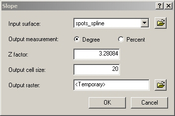
(The instructions for this lab
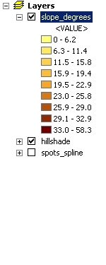
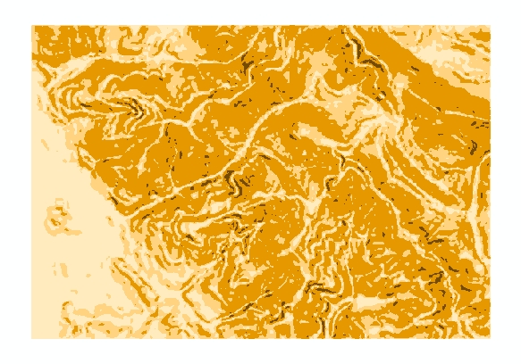
forgot to do this, so the slope was severely underestimated.) Below, the slope in degrees is overlaid on a hillshade, which helps the human eye
to recognize ridges and valleys.
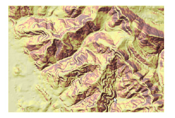
What causes the light-colored ribbons, for example at the arrow in the lower right? They coincide with roads; I wonder if they are
artifacts of digitizing the paper map, where the road symbols obscured the
contour lines. Or maybe they show manmade cuts and fills that created flat
roads.
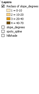
For future calculations, we can classify the slope values into classes relevant to landslide
hazards. ArcMap displays the classes with random colors by default; I reset the
colors to make a sequence from lighter to darker.
Recall that in the last lab, the soigeohy layer was created by
geology layer with slope
stability of "poor". In fact, "poor" stability was found
only in the Orinda Formation, which is notorious for landslides because of its
weak conglomerate rocks: see this discussion
of mapping landslide hazards from the USGS, and the explanation of local
geology in this excerpt from the Strawberry
Creek Management Plan.soils layer, to obtain the attributes
of the soils.Soon we'll do analogous operations on rasters. But first, since the soigeohy
layer has already been constructed, we convert it to a raster. The values in the
new raster are taken from one of the fields of the polygon layer
attribute table. We use the SOILTYPE field because it classifies the soils and
determines all their physical properties, such as pH, etc. Then this field can
be used to join to the rest of the attribute table.
The raster covers a rectangle just large enough to include all the polygons
(as selected in the Spatial Analyst > Options > Extent tab); cells in the rectangle but outside the polygons contain a code for
"no data".
A buffer of 150 feet around the roads is created by using (1) Distance > Straight Line with the roads feature layer, then (2) Raster Calculator to select cells with distance <= 150 feet, producing values of 0 (false) and 1 (true).
Also, I decided that since landslides happen on the surface, the roads in tunnels should be omitted. I looked in the Attribute Coding Standards for Digital Line Graphs to find the code for tunnel, MINOR2 = 0601; selected roads that did not have this code; and exported the selection, and used this shapefile for the distance calculation.
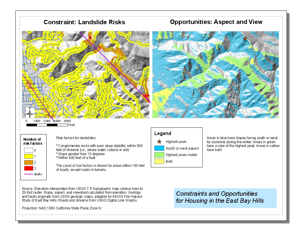
We want to locate areas of landslide danger, which is defined as having all three risk factors:
One way to do this is to multiply the reclassified slope by the roads
buffer, which sets all values outside the buffer to 0 and leaves others
unchanged, and then select cells with slope class ≥ 2 and valid
data in the soigeohy layer. (I don't see a function for valid data
in the Raster Calculator, but selecting values ≥ 1 will work.) Another way is to apply all
three conditions at once:
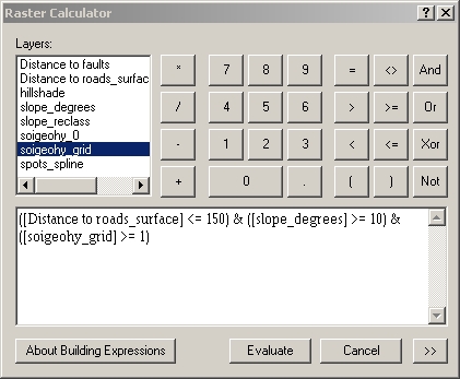
Areas with all three risk factors are shown in red:
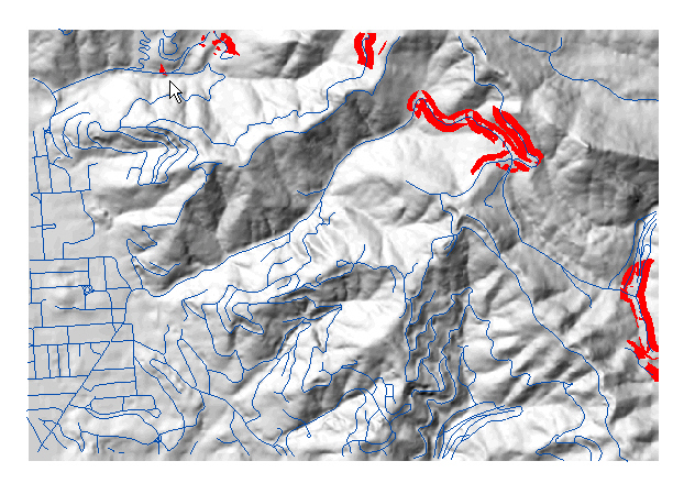
In some of these areas, such as around Grizzly Peak Boulevard, the road is on
the ridge line and the landslide would actually flow down away from the road, so
maybe this area isn't such a concern. Or would a landslide flowing away from the
road make the roadbed collapse? The greatest danger would be where the landslide
would flow down onto the road and block it, such as on Centennial Drive, in the
upper left where the arrow points. Highway 24 is the worst problem, because of
its heavy traffic; landslides have already hit Highway
24 and the Orinda BART station.
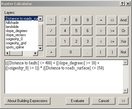
The lab assignment asks us to create a buffer zone within 400 feet of the faults, and to consider this as an additional landslide hazard zone. I decided to make a map showing areas with any of the risk factors
This is like doing a union of the three areas. More specifically, I would
like to calculate how many risk factors are present. To do the calculation,
first I have to replace "nodata" values in the soigeohy
layer with 0, using Reclassify. Also, let's suppose we only care about
landslides that threaten homes and roads, so I'll clip the areas to the roads
buffer layer, since homes are near roads. Here's the expression to be
calculated:
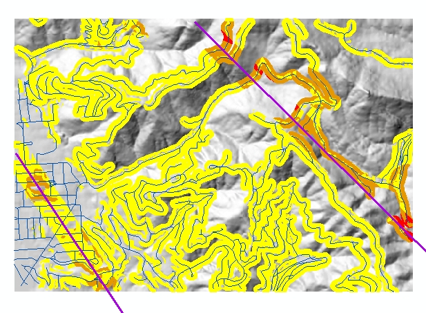
And this is the result. The slope is steeper than 10 degrees throughout most of
the hills, so most of the roads are surrounded by zones with at least this one
risk factor. Around the Hayward Fault, on the left, the fault is one risk factor
and the slope is a second risk factor in a few areas. The Wildcat Fault, on the
right, runs through steeper terrain, so there are two risk factors around most
of it, plus the third factor of geology in the red spots.
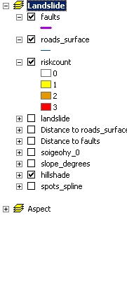
The city might, for example, regulate construction tightly where there are one or more risk factors, and ban housing altogether where there are two or more. It would also be useful to take into account the soil type and soil permeability.
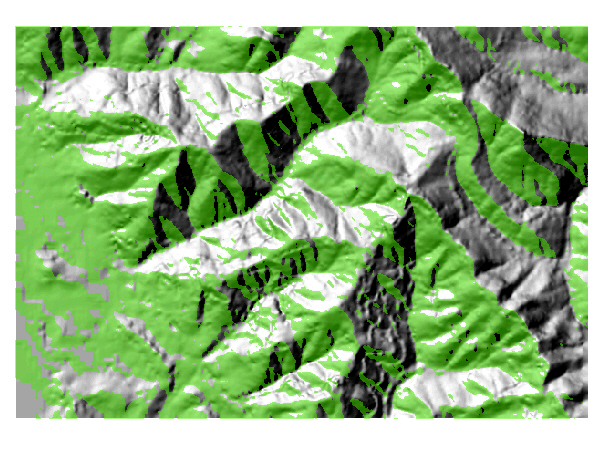
I would like to live in an energy-efficient house that gets warmth from
sunshine during the winter. South and west-facing slopes would be good;
east-facing slopes will tend to be overshadowed by the hills to the east. I used
the Aspect tool to calculate aspects of the interpolated elevation, then used
the Raster Calculator to select aspects in the south, southwest, and west range:
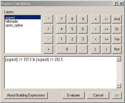
Here's the result, shown in green:
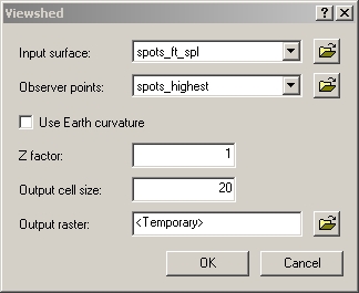
I experimented a little bit with viewsheds. It's possible to calculate viewsheds of lines or points, but calculating viewsheds of a lot of lines, such as the entire roads layer, takes forever. I tried calculating viewsheds of just a few points, by selecting a few spots from the spots layer and exporting them as a layer, but it refuses to use a Z factor greater than 1; it was necessary to change the values in the spots field to convert them from meters to feet so the Z factor would be 1.
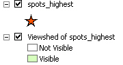
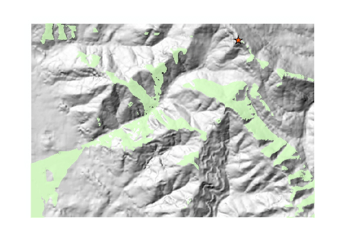
Let's suppose I would like to see the highest peak in the area. I selected
one of the spots at the highest level, exported it to a layer, and calculated
its viewshed:
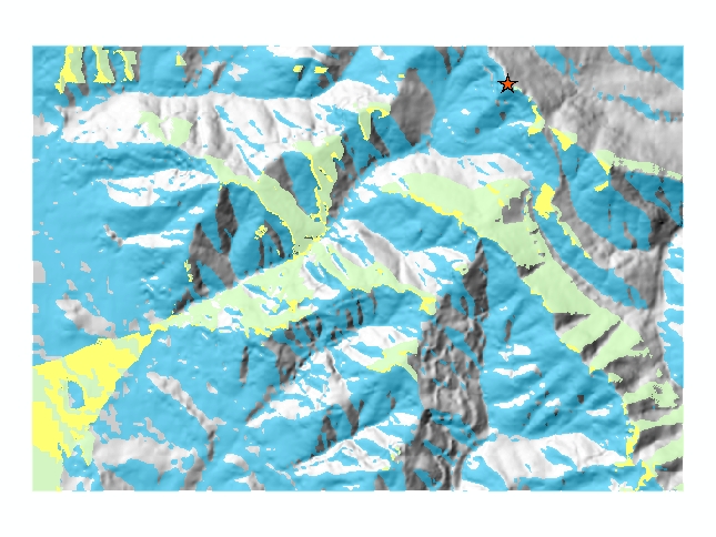
Finally, let's combine these two opportunities with the raster calculator, to
find areas with both good aspects and good views:
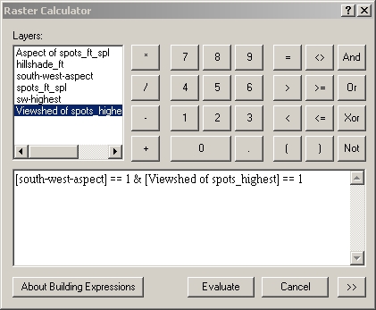
Here's the result, with the good aspects in blue, the good view in green, and
the overlap in yellow.
Finally, it's time for a map layout to explain the results. I thought that
showing both constraints and opportunities on the same map would be too
complicated, so I opted for two maps side by side on a landscape oriented page.