My New House Site in Claremont Canyon

Well, I personally would not live in Claremont Canyon; I want to live in the middle of the city near shopping, entertainment and BART, and without a long uphill commute every day. But let's pretend I'm a real estate agent for somebody who loves living up on the hill with nice views. I will present my client with some opportunities:

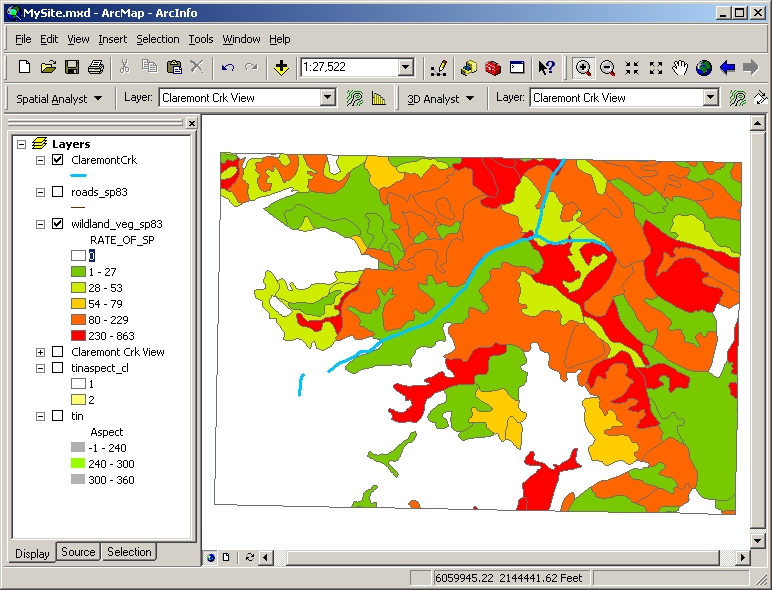
1. View: Suppose the client likes to look at Claremont Creek. I selected the line features that make up the creek from the hydrology layer, exported them as a layer, and used Surface Analysis > Viewshed on the 3D analyst toolbar to define a viewshed with the TIN surface. It takes too long to calculate with the default resolution, so I increased the cell size to 100 feet.
   
   I'll use ArcMap for the analysis instead of ArcScene, because ArcScene can't turn on the Spatial Analyst toolbar with the Raster Calculator. Also, the 2D display will show the whole study area, whereas in the 3D display, some parts might be hidden behind hills. The viewshed is shown with transparency over the TIN, which has hillshading turned on.
   
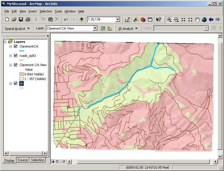
   The values symbolized as "visible" are actually integers ranging from 1 to 357; I'm guessing these are the number of vertices on the line features that are visible.
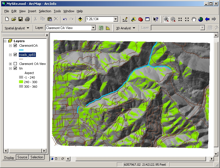
2. Aspect: Suppose the client likes to get afternoon light and look at sunsets. At our latitude, the sun sets at azimuths ranging from about 240 degrees in winter to about 300 degrees in summer (270 degrees is due west). I classified the aspects of the TIN using the Layer Properties dialog, Symbology tab, Classify button; here the desirable aspects are shown in green.
   
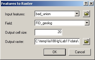
3. In order to overlay these layers with other feature layers, they must be converted to the same data model, either raster or vector. I tried converting the TIN aspect to polygons, but the file was large and slow to display, probably because there are so many complicated polygons. Therefore, I converted the TIN aspect to a raster (from the 3D Analyst toolbar), using a cell size of 20 feet since that was used in the previous lab.
   
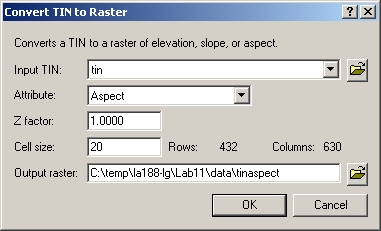
   The output raster contains the exact aspect in degrees, but only a classification is needed, so I used Reclassify on the 3D Analyst toolbar to replace the values with 0 (outside desired range) and 1 (inside).
   
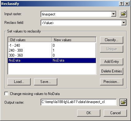
   This reduces the file size from 1.72 MB to 88 KB.

I will also warn the client about natural hazards, which create constraints, for example:

1. Fire: I used the rate-of-spread field in the wildland vegetation layer as an indicator of fire danger. (Caution: the value of 0 in the white polygons does not mean that fire won't spread there. It means that the fuel model in these areas is residential, not wildland vegetation, and therefore they were not included in this layer. See the background on the East Bay Hills Fire Study. If I had a real client, I would have to find the Fire Study maps for those areas too.)
   
   I arbitrarily decided that the yellow, orange and red areas (rate of spread greater than 53 feet per minute) were too dangerous, selected those polygons, and created a layer from them (right-click original layer, point to Selection > Create Layer from Selected Features).
2. Landslide: In the geology layer, I selected polygons with "poor" slope stability ( a simplification of the analysis in Lab 10).
3. Earthquake: I added the faults layer, and created a buffer of 400 feet around the faults, as in Lab 9.
4. I made a union of all the constraints, using ArcToolbox, Analysis Tools > Overlay > Union.
   
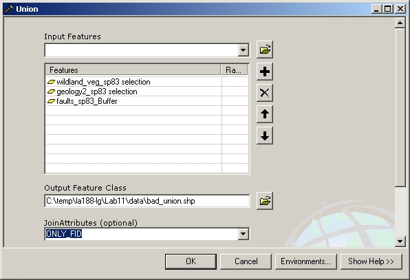
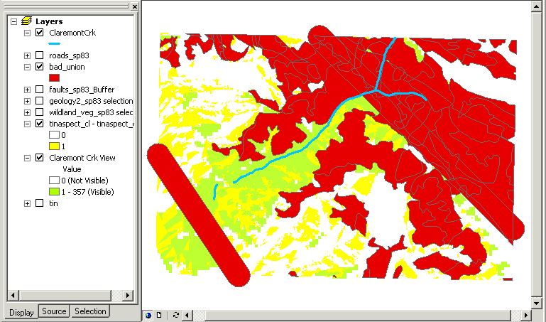
   I chose not to join the attributes of the original layers, since I'm not using them. Here's the union of all the "bad" areas (red), shown along with the "good" areas (yellow and green); roads and hillshade have been removed because the map was too messy. The fire constraint has eliminated some of the formerly desirable area on the south side of Claremont Canyon; the landslide and faults constraints eliminated the upper end of the canyon.
   

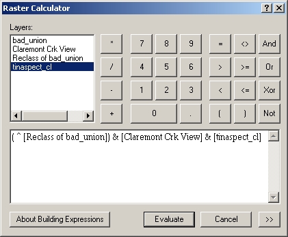
Finally, I'll make a summary for the client combining the "good" and "bad" criteria. I converted the "bad" union layer to a raster, using a cell size of 20 feet as before; it doesn't matter what field is used for the value, since I just need to distinguish between data and no data.

In order to use the Raster Calculator, I had to reclassify this raster so that No Data (cells outside of the "bad" polygons) became 0, and all the real data values were nonzero. Then I used the Raster Calculator to select cells that have good view, good aspect, and none of the constraints.

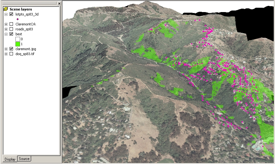
To make an exciting presentation for the client, I'll display the resulting best areas in ArcScene, on top of an aerial photograph draped over the TIN (this photograph takes an agonizingly long time to download, unzip, make pyramids, and load into ArcScene). Here's a view looking up beautiful Claremont Canyon. The green parts are the recommended areas, and the pink spots are locations of existing houses. Perhaps the client would like to bid for an existing house in a green area; the green areas that don't have houses are pretty much all owned by the university or the park district, so it would be hard to get hold of them. Notice that the Claremont Hotel (large white building at lower right) is sitting on a nice spot, and probably owns the nice area behind it. It would be great to live at the hotel; it's even on bus routes.