Extreme Value Theory 2: The family of extreme value distributions
Contents
The Type I domain
The importance of the Gumbel distribution is that it applies to more than just exponential random variables. In fact, there are only three possible forms for the limiting distribution of the maximum, which are known as type I, II and III, or Gumbel, Frechet and Weibull distributions. See Castillo (1988) chapter 3 for many examples and a table of which of these types results from some common parent distributions.
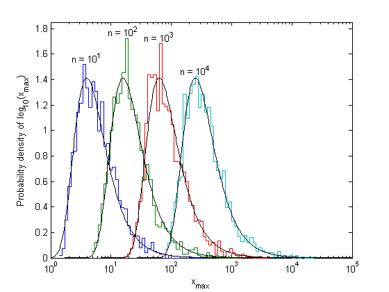
Distributions whose tails decrease exponentially produce a Type I distribution of the maximum. Besides the exponential distribution, this class includes the normal distribution and many others. Here is an example of block maxima of normal random variables.
Ntrials = 2000;
n = 10.^(1:4);
Nhist = 50;

for k = 1:length(n)
    xmax = max(randn(n(k),Ntrials));
    [count,xout] = hist(xmax,Nhist);  dx = xout(2)-xout(1);
    f = count/Ntrials/dx;  % Probability density
    stairs([xout-dx/2 xout(end)+dx/2],[f f(end)]), hold all
    [m,xm] = max(f);  m = min(m,1.6);  yl = ylim;
    text(xout(xm)-.05,m,sprintf('n = 10^{%d}',log10(n(k))),'horiz','r')
end, hold off, set(gca,'ylim',[0 max(yl(2),1.65)])

xlabel('x_{max}'),ylabel('Probability density')
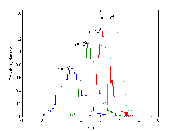
This distribution is converging to the Gumbel distribution, although it is much harder to prove than it was for the exponential. As well as marching to the right, the peaks also get narrower with larger n. This is because the normal density decreases faster than the exponential density, so it is less likely to produce very high values. In order to get a universal form, Xmax(n) must be both centralized and scaled. Define the standardized variable
whose cumulative distribution will be given by

As before, the peak of the pdf for Xmax(n) is located at the point where the probability of exceedance for a single variable is 1/n, and the expected number of exceedances in n samples is 1:
The scale factor, a(n), can be defined as the increase in x corresponding to an increase in u from 0 to 1. Thus
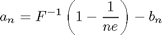
These formulas are not unique, and variations can be found, as long as they also work as n goes to infinity. The next figure shows the Gumbel distribution with these location and scale parameters and the observed histogram.
b = norminv(1-1./n,0,1); % inverse cdf from Statistics Toolbox
a = norminv(1-1./(n*exp(1)),0,1) - b;
x = linspace(0,max(xout)+0.5,500);
for k = 1:length(n)
    line(x,evpdf(-x,-b(k),a(k)),'color','k')
    % or exp(-(x-b)/a - exp(-(x-b)/a))/a
end
For large n there is an approximation for the inverse cdf using an asymptotic form of inverse erf, found e.g. at Wolfram Functions. This can be used to get an asymptotic expression for a and b,

as in de Haan and Ferreira, Example 1.1.7.
The Type II domain: heavy-tailed distributions
The second type of extreme value distribution occurs when the parent distribution is "heavy-tailed", that is, it decays as a power law, slower than exponential, and therefore has infinite moments. Again if the survival function, 1-F(x), has a simple form, it will be easy to find the limiting distribution of the maximum. The most famous example is the Pareto distribution:

Note the relation to the exponential distribution function: if x is Pareto-distributed, then y = alpha*log(x) has a standard exponential distribution.
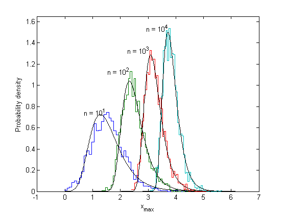
Pareto distributions produce outcomes that are mostly near the left boundary, with a few extreme values that are very far out. Therefore, the distribution of the maximum of a set of Pareto variables can be seen more clearly by calculating the histogram of log(Xmax) rather than Xmax directly.
A = 5/3;
for k = 1:length(n)
    xmax = max(rand(n(k),Ntrials).^(-1/A)); % uses less memory than gprnd
    [count,xout] = hist(log10(xmax),Nhist);  dx = xout(2)-xout(1);
    f = count/Ntrials/dx;  % Probability density of log10(x)
    stairs(10.^[xout-dx/2 xout(end)+dx/2],[f f(end)]), hold all
    m = max(f);
    text(n(k)^(1/A),m+.05,sprintf('n = 10^{%d}',log10(n(k))),'hor','c')
end, hold off, set(gca,'xscale','log'), axis([xlim 0 1.85])

%title(sprintf('Observed maximum of n Pareto variables, \\alpha = %.2f',A))
xlabel('x_{max}'),ylabel('Probability density of log_{10}(x_{max})')
The distribution of the logarithm of Xmax(n) looks just like the distribution of the maximum of exponential random variables: it has a fixed shape and moves to the right, with the location of its peak proportional to log(n). Since adding a fixed amount to log(Xmax) corresponds to multiplying Xmax by a fixed amount, the movement can be described using a scale factor, instead of a location factor. The appropriate scale factor is again the location of the peak of the histogram, which is the point where the probability of exceedance is 1/n:
Then the limiting distribution function for the scaled variable U = Xmax/a(n) will be

This limiting distribution is called the Frechet distribution, or Type II extreme value distribution. Unlike the Type I distribution, this one has a shape parameter, alpha, which depends on the parent distribution, and it has a left boundary instead of being defined for all u. Also, this limit could have been derived directly by plugging y = alpha ln(x) into the Type I distribution.
Compare this limiting distribution to the observed distribution of the maximum:
x = logspace(0,5,500);
for k = 1:length(n)
    f = gevpdf(x,1/A,n(k)^(1/A)/A,n(k)^(1/A));
    % or exp(-n(k)*x.^-A).*(x.^-(1+A))*n(k)*A
    line(x,f*log(10).*x,'color','k') % pdf of log10(x)
end
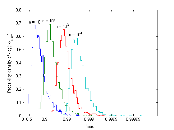
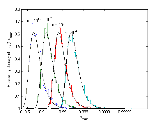
The Type III domain: right-bounded variables
The last type of extreme value distribution occurs where the parent distribution is bounded on the right, such as the Beta(1,alpha) distribution, where

(alpha = 1 gives the uniform distribution). The maximum can never exceed the boundary, and the distribution of the maximum squeezes up toward the boundary, getting narrower as n gets larger. The behavior within the narrow region near the boundary can be seen by taking the histogram of -log(1-x) intead of x.
for k = 1:length(n)
    xmax = max(betarnd(1,A,n(k),Ntrials));
    [count,xout] = hist(-log(1-xmax),Nhist);  dx = xout(2)-xout(1);
    f = count/Ntrials/dx;  % Probability density of -log(1-xmax)
    stairs([xout-dx/2 xout(end)+dx/2],[f f(end)]), hold all
    [m,xm] = max(f);
    text(log(n(k))/A,m+.03,sprintf('n = 10^{%d}',log10(n(k))),'hor','c')
end, hold off, axis([xlim 0 0.8])

xtick = [0 .5 .9 .99 .999 .9999 .99999];
set(gca,'xtick',-log(1-xtick),'xticklabel',xtick)

%title('Observed maximum of n beta-distributed variables')
xlabel('x_{max}'),ylabel('Probability density of -log(1-x_{max})')
The appropriate location parameter is the right boundary,
and the scale parameter is the distance of the peak of the histogram from the right boundary,

Thus the scaled variable is U = (Xmax - b(n))/a(n) (note that U <= 0), and its limiting distribution function is

This limiting distribution is called the maximal Weibull, or type III extreme value distribution. This limit could also have been derived by observing that y = -alpha ln(1-x) has an exponential distribution, and plugging it into the Type I distribution.
x = 1-logspace(0,-5,500);
for k = 1:length(n)
    f = gevpdf(x,-1/A,n(k)^(-1/A)/A,1-n(k)^(-1/A));
    % or exp(-n(k)*(1-x).^A).*((1-x).^(A-1))*n(k)*A
    line(-log(1-x),f.*(1-x),'color','k') % pdf of -log(1-x)
end
The generalized extreme value distribution (von Mises form)
All three types of extreme value distribution can be expressed in a single equation:

where K=0 for type I, K>0 for type II, and K<0 for type III. K is called the extreme value index, or shape parameter; mu and sigma are location and scale parameters, unfortunately not the same as the b(n) and a(n) defined above.
x = linspace(-3,3,500)'; clear xt; styles = {'-',':','--','-.','-'};
K = [-4 -1 0 1 4];  sigma = 1;  mu = 0;
for k = 1:length(K)
    plot(x,gevcdf(x,K(k),sigma,mu),styles{k}), hold all
    if (K(k) < 0)
        yt = 0.9;   xt = gevinv(yt,K(k),sigma,mu) + 0.05;
    else
        xt = 2.3;   yt = gevcdf(xt,K(k),sigma,mu);
    end
    text(xt,yt,sprintf('K = %g',K(k)),'hor','l','ve','top');
end, hold off
axis([xlim -.01 1.01])
xlabel('(x-\mu)/\sigma'), ylabel('cdf H(x)')
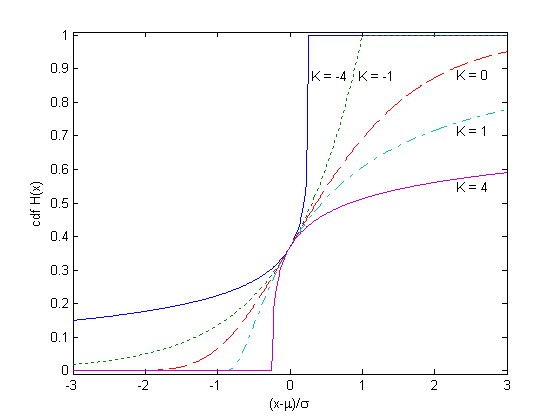
The distribution has a finite left boundary for K>0, a finite right boundary for K<0, and extends to infinity in both directions for K=0. According to the extremal types theorem, if the limiting distribution of the maximum exists, it must have this form.
Determining the domain of attraction
There are several tests for determining the domain of attraction and shape parameter of a given parent distribution. They all depend on the behavior of the parent distribution in the tail. One that is relatively easy to apply is the Pickands test, which states that if
then the limiting distribution has shape parameter K. This test can be thought of as expressing the cost of decreasing risk. For example, think of x as the height of a sea wall, and 1-F(x) as the probability that waves exceed the height x in a given year. Then the bottom of the fraction is the increase in height that is needed to cut the risk of exceedance in half, from epsilon to epsilon/2; the top is the second increase needed to cut the risk in half again, from epsilon/2 to epsilon/4. If the second increment in x is the same as the first, the ratio equals 1 and K=0 (Gumbel domain); if it is greater, the ratio is greater than 1 and K>0 (Frechet domain); and if it is smaller, the ratio is less than 1 and K<0 (Weibull domain).
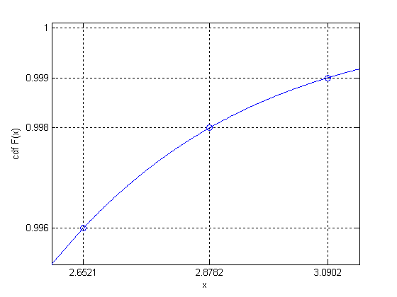
This limit can be evaluated analytically, given the parent distribution. The figure below shows an example of the two intervals of x where the parent distribution is normal, as the probability of exceedance is decreased from epsilon = 0.004 to 0.002, and then to 0.001. The two intervals are approximately equal, and their ratio will go to exactly 1 as epsilon goes to zero: therefore the distribution is in the Gumbel domain.
ep = 4e-3;
ytick = [1-ep 1-ep/2 1-ep/4 1];
xt = norminv(ytick(1:3),0,1);  marg = (xt(2)-xt(1))/4;
x = linspace(xt(1)-marg,xt(3)+marg,500);
plot(x,normcdf(x,0,1),'b-',xt,ytick(1:3),'bo'), grid on, axis tight
yl = ylim; set(gca,'ylim',[yl(1) 1.0001])
set(gca,'xtick',xt,'ytick',ytick)
ylabel('cdf F(x)'), xlabel('x')