Extreme Value Theory 1: Introduction

Contents

The distribution of the maximum

The Central Limit Theorem describes the pdf of the mean of a large number of iid random variables: for large n, the pdf of the mean approaches a Gaussian, no matter what the parent distribution was (as long as it had finite variance). There is an analogous result for the maximum: its pdf also will approach a limiting form.

The limiting distribution can be investigated experimentally by finding the maximum of a sample of random variables, repeating for many samples, and constructing a histogram. A larger sample is likely to have a larger maximum, so the histogram marches to the right with increasing sample size. In the figure below, the stairstep line is the histogram of the maximum of n random variables, which were exponentially distributed with mean = 1.

Ntrials = 2000;
n = [10 100 1000 10000];
Nhist = 50;

for k = 1:length(n)
    xmax = max(exprnd(1,n(k),Ntrials),[],1);
    [count,xout] = hist(xmax,Nhist);  dx = xout(2)-xout(1);
    f = count/Ntrials/dx;  % Probability density
    stairs([xout-dx/2 xout(end)+dx/2],[f f(end)]), hold all
    [m,xm] = max(f);
    text(log(n(k)),m+.02,sprintf('n = 10^{%d}',log10(n(k))),'horiz','c')
end, hold off, axis([0 18 0 0.5])

xlabel('x_{max}'), ylabel('probability density')
% title('Observed maximum of n exponentially distributed variables')

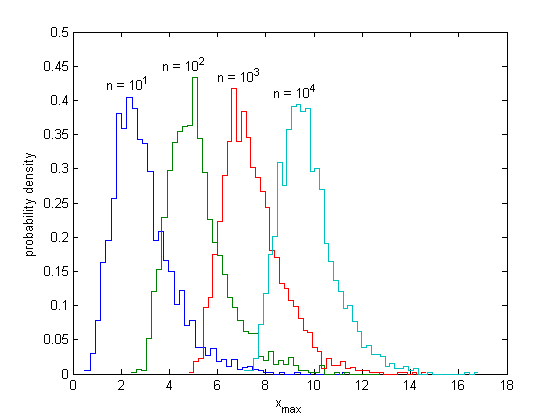
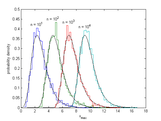
We will show below that all these distributions are approaching the same curve, each shifted to the right. The limiting curve is called the Gumbel distribution, or type I extreme value distribution.

x = linspace(0,max(xout),500);
for k = 1:length(n)
    line(x,gevpdf(x,0,1,log(n(k))),'color','k')
    % Matlab <7: use   n(k)*exp(-x).*exp(-n(k)*exp(-x))
end

Derivation of the limiting distribution

The distribution appears to be marching to the right with the same displacement for each factor of 10 increase in n; the peak of each curve occurs at ln(n). We can prove that this is correct. The cumulative distribution function for the exponential distribution is

and the cumulative distribution for the maximum, Xmax(n), is just the probability that all of the n variables are less than x, so

The distribution function for the centralized variable U, defined as Xmax(n)-ln(n), is

The peak location, at x = ln(n), is also the location where the probability of exceeding x in one trial is 1/n, and the expected number of outcomes exceeding x in n trials is 1. The limiting distribution is shown in detail below.

u = linspace(-5,5,500);
[hax,h1,h2] = plotyy(u,evpdf(-u,0,1),u,1-evcdf(-u,0,1));
ylabel(hax(1),'probability density'),grid on; set(h1,'linestyle','--')
set(gca,'defaulttextcolor',get(gca,'ycolor'))
text(-1,0.3,'f(u) = e^{-u}exp(-e^{-u})','horiz','r','backg','w')
text(-log(log(2)),log(2)/2,'\leftarrow median','rot',45)
mu = -psi(1); text(mu,exp(-mu-exp(-mu)),'\leftarrow mean','rot',45)

axes(hax(2)), ylabel('cumulative probability')
text(2,0.83,'F(u) = exp(-e^{-u})','color',get(gca,'ycolor'),'back','w')

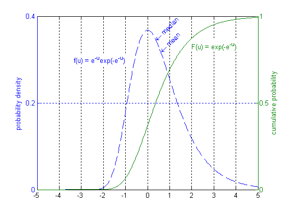
For negative u, exp(-u) quickly goes to infinity, so F(u) quickly goes to 0; for positive u, exp(-u) slowly goes to 0, so F(u) slowly goes to 1. The pdf is skewed right, because a high maximum needs only one of the outcomes to be very high, but to get a low maximum all of them must be low.

Next: The family of extreme value distributions

Published with MATLAB® 7.3