Extreme Value Theory 4: Fitting Distributions to Data

Contents

Unknown parent distribution

The true usefulness of the extreme value distribution is to fit data where the parent distribution is unknown. For example, there may only be records of the maximum flow of a river each year, not the flow every day or every hour. Regardless of what the overall distribution of flows was, the distribution of extreme flows must take the form

for some values of the parameters K, mu, and sigma. One way of estimating these parameters is the maximum likelihood method, which finds the parameter values which maximize the probability of generating the observed data set. The Statistics Toolbox provides functions to do this for many probability distributions, including the generalized extreme value distribution.

Testing the gevfit function

Given a data set, gevfit returns estimates for K, mu, and sigma. Let's see what it does with maxima generated from a parent normal distribution, which we know should give an extreme value distribution with K=0. Each data point is the maximum of 10,000 samples from a normal distribution.

blocksize = 1e4; Ntrials = 500;
xmax = max(randn(blocksize,Ntrials));
[paramEsts,paramCIs] = gevfit(xmax);
kMLE = paramEsts(1) % Shape parameter
sigmaMLE = paramEsts(2) % Scale parameter
muMLE = paramEsts(3) % Location parameter

kMLE =

   -0.0311


sigmaMLE =

    0.2517


muMLE =

    3.7269

These are the maximum-likelihood estimates; let's also look at the 95% confidence intervals:

kCI = paramCIs(:,1)
sigmaCI = paramCIs(:,2)
muCI = paramCIs(:,3)

kCI =

   -0.0893
    0.0271


sigmaCI =

    0.2348
    0.2697


muCI =

    3.7024
    3.7514

The maximum-likelihood method tends to give biased results, as can be seen in this example, where the estimate of the shape factor K is usually negative. Depending on the sizes of the blocks and number of blocks, the correct value (zero) may not even be inside the 95% confidence interval. This can happen because you don't actually get the extreme value distribution unless the block maximum is taken over large enough blocks. "Large enough" depends somewhat on the parent distribution; the distribution of the maximum approaches the extreme value distribution very quickly if the parent is exponential (block size of 100 is good enough) but much more slowly if the parent is normal (block size must be 10,000 or more). You can experiment with different block sizes and different parent distributions.

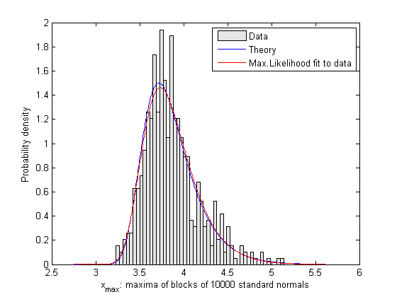
Still, the fitted distribution is close to the theoretically expected distribution, as shown in the next plot. (The formulas for the location and scale factors from the previous notes are used. Recall that the peak is at the point where the probability of exceeding it is 1/n in the parent distribution.)

[count,xout] = hist(xmax,50);  dx = xout(2)-xout(1);
h = bar(xout,count/Ntrials/dx,1); set(h,'facecolor',[.9 .9 .9])
b = norminv(1-1/n,0,1); a = norminv(1-exp(-1)/n,0,1) - b;
x = linspace(min(xout)-0.5,max(xout)+0.5,500)';
line(x,gevpdf(x,0,a,b),'color','b')
line(x,gevpdf(x,kMLE,sigmaMLE,muMLE),'color','r')
legend('Data','Theory','Max.Likelihood fit to data')

xlabel(sprintf('x_{max}: maxima of blocks of %d standard normals',n))
ylabel('Probability density')

Exceedance

Our real goal is not to get an exact value for K, but to answer questions about the maximum values that may occur in the future. For example: The Dutch government requires the sea wall to be high enough that the probability that the maximum wave height exceeds it in a given year is 0.0001. What should the height be? This is also called the "return level", the level that is expected to be exceeded once in 1000 years. Suppose we only have observations of maximum wave height each year for 100 years. Is it possible to answer the question? Yes: first fit the data to a generalized extreme value distribution. Then the return level exceeded once in m years, R(m), is the x such that

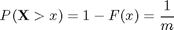
which is given by the inverse distribution function,

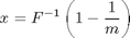
The Statistics Toolbox provides this inverse function.

m = 1000; % exceedance once in M years
R_MLE = gevinv(1-1/m,kMLE,sigmaMLE,muMLE)

R_MLE =

    5.2913

Uncertainty of return values

Since we can't estimate the shape, location and scale parameters with perfect accuracy, we can't compute the return level with perfect accuracy either. What range of R is consistent with the data? Answering this question involves searching the high-likelihood region of parameter space for the highest and lowest values of R. For further discussion of how to do this, see the Matlab demo, showdemo gevdemo.

Published with MATLAB® 7.3